Quick Start
This section provides a quick guide to preparing the required input files for colocalization analysis with LocusFocus.
Up to three files may be selected and uploaded, with a maximum combined file size of 100MB:
.txt or .tsv (required): tab-separated primary summary statistics (eg. GWAS)
.ld (optional): PLINK-generated LD matrix – must have the same number of SNPs as primary file
.html (optional): Secondary datasets to test colocalization with.
For uploaded secondary datasets, each data table must be preceded by an <h3> title tag describing the table
You may use the merge_and_convert_to_html.py script to ready your files for uploading
Press and hold the Ctrl/Cmd key to select multiple files
Selecting the human coordinate system
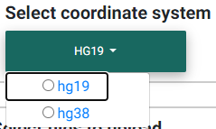
Selecting the appropriate human genome coordinate system.
Before you begin, you must choose the appropriate human coordinate system for accurate visualization of the data in the colocalization plot, accurate matching with GTEx data (if selected), and accurate matching with the 1000 Genomes data for LD calculations (unless a custom matrix is uploaded). hg19 refers to the GRCh37 and hg38 to the GRCh38.
You may ignore this step if your purpose is to simply compute the colocalization between two datasets that you upload. In that case, simply ensure the secondary dataset(s) have been prepared using the merge_and_convert_to_html.py script or the merge_and_convert_to_html_coloc2.py script if also running COLOC2.
Primary dataset input
Please note that use of the web tool requires uploading your summary statistics to a public server.
The primary dataset will usually be a genome-wide association study (GWAS) file with summary statistics. You may download our sample dataset for meconium ileus around SLC26A9 gene.
A tab-delimited text file input is preferred.
The first few lines of a sample input file are shown below.
> head MI_GWAS_2019_1_205500-206000kbp.tsv

#CHROM       BP      SNP     REF     ALT     BETA    SE      P       AF      N
1    205500022       rs114114637     C       A       -0.0739321001603956     0.152350860711495       0.627481118153097       0.0260753323485968      6770
1    205500203       rs11240506      A       T       -0.028580509980184      0.0720691836942088      0.691684232909143       0.123175036927622       6770
1    205500342       rs76069011      C       T       0.269353170260049       0.246838504548712       0.275179551742949       0.0104350073855244      6770
1    205500450       rs45495498      C       G       -0.253245978881793      0.252113050092583       0.31514069034813        0.0127828655834564      6770
1    205500543       rs11240507      T       C       0.0546597433178092      0.0555106475800506      0.324785538604616       0.256992614475628       6770
1    205500586       rs146709978     C       G       0.184819472593451       0.219156490990298       0.399048427185569       0.0155140324963072      6770
1    205500719       rs74142375      T       A       0.312872957911176       0.227488579712488       0.169027675607645       0.013301329394387       6770
1    205500767       rs3838999       G       GA      -0.0717111663499279     0.152168074740335       0.637453014437489       0.0259283604135894      6770
1    205500829       rs3795547       C       T       -0.00434473636812393    0.12753158044846        0.972822985458176       0.0379985228951256      6770
Simple Sum Colocalization
For the Simple Sum method, two columns are absolutely necessary:
ID - The SNP rs id or chrom_pos_ref_alt_build format (e.g. 1_205860191_A_G_b37).
P - The association p-value
In this case, you must check the box “Use marker ID column to infer variant position and alleles” to map the provided rs ID’s to the chromosomal position and alleles using dbSNP.
Alternatively, for more accurate matching of alleles, all four fields (chromosome, basepair position, reference and alternate alleles) may be provided in addition to the ID column field.
ID - The SNP rs id or chrom_pos_ref_alt_build format (e.g. 1_205860191_A_G_b37)
#CHROM - The chromosome column (either “X” or “23” is acceptable)
POS - The basepair position (in hg19 coordinates)
REF - The reference allele (on the plus strand, as defined in the 1000 Genomes)
ALT - The alternate allele (on the plus strand, as defined in the 1000 Genomes)
P - The association p-value
Use the web form to change the column names as found in your file if different from the default names. For the example above, you would change the position column default name (POS) to BP and MAF to AF.
COLOC2 Colocalization
To run COLOC2, check the box “Add required inputs for COLOC2”. For this option, additional fields are required, and the corresponding required fields will be populated to allow for input of the column names if other than default:
BETA - The beta of the SNP in the association analysis
SE - The standard error of beta
N - The total sample size of the study
MAF - The minor allele frequency
Study type - Select either quantitative or case-control.
For the case-control case, you are required to provide the number of cases in the study.
If you have a csv or excel file, see below on how to convert it to a tab-delimited file.
We recommend having a dense set of SNPs for the region in order to obtain accurate results. If the number of SNPs in the region of interest is too small, it may not be possible to compute the Simple Sum p-value.
Formatting the primary dataset file input
The simplest way to convert either csv or excel file formats is to open the file in Excel, then choose to save the file as a tab-delimited file.
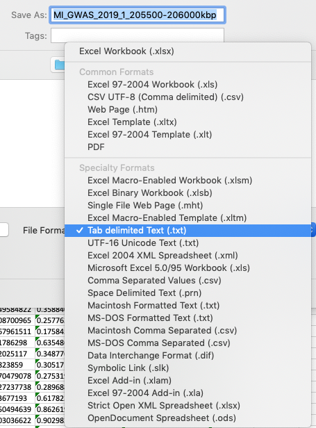
Formatting your csv or Excel file as a tab-delimited file using Excel.
Non-default column names
Use the web form to change the column names as found in your file if different from the default names. For the example above, you would change the position column default name (POS) to BP and MAF to AF.
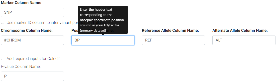
Changing default column names to correspond to input file header names.
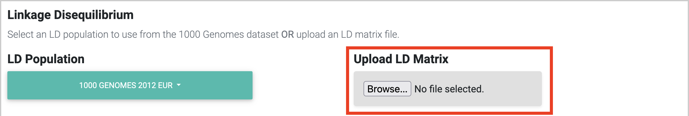
Selecting an LD matrix
You may either:
For the most accurate colocalization statistics, we recommend uploading the LD matrix of your study. If this is unavailable, you may select the most appropriate 1000 Genomes population subset for your study.
Note: for X chromosome datasets in hg38 coordinates, LocusFocus will only select female samples from the selected 1000 Genomes population. This is to account for an issue with LD calculation with PLINK in this specific case.
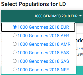
Selecting a publicly available 1000 Genomes population LD matrix
hg19

Selecting the most appropriate 1000 Genomes population (hg19).
These datasets were obtained from LocusZoom. However, for more accurate results, we suggest computing and uploading the LD matrix for your GWAS study.
The 1000 Genomes population dataset (phase 1, release 3) consists of:
EUR: European population of 379 individuals
85 CEU - Utah Residents (CEPH) with Northern and Western European Ancestry
93 FIN - Finnish in Finland
89 GBR - British in England and Scotland
14 IBS - Iberian Population in Spain
98 TSI - Toscani in Italia
AFR: African population of 246 individuals
61 ASW - Americans of African Ancestry in SW USA
97 LWK - Luhya in Webuye, Kenya
88 YRI - Yoruba in Ibadan, Nigeria
ASN: Asian population of 286 individuals
97 CHB - Han Chinese in Beijing, China
100 CHS - Southern Han Chinese
89 JPT - Japanese in Tokyo, Japan
AMR: Ad Mixed American population of 181 individuals
60 CLM - Colombians from Medellin, Colombia
66 MXL - Mexican Ancestry from Los Angeles USA
55 PUR - Puerto Ricans from Puerto Rico
Descriptions of the population codes can be found in the IGSR: The International Genome Sample Resource. Also, please note that the known cryptic relationships in the 1000 Genomes were not removed for the non-European populations.
hg38
Selecting the most appropriate 1000 Genomes population (hg38).
The hg38 version of the 1000 Genomes population is computed from a fully realigned call set against GRCh38. The biallelic SNV call set is used and more details are available on the 1000 Genomes Project FTP site.
A total of 2,548 individuals are available on the 1000 Genomes, and 2,507 have been assigned a population and super-population code. The distribution of populations available for selection on the app are as follows:
EUR: European population of 502 individuals
99 CEU - Utah Residents (CEPH) with Northern and Western European Ancestry
89 GBR - British in England and Scotland
107 IBS - Iberian Population in Spain
111 TSI - Toscani in Italia
96 FIN - Finnish in Finland
NFE: Non-Finnish European (406 individuals)
AFR: African population of 671 individuals
97 ACB - African Caribbeans in Barbados
61 ASW - Americans of African Ancestry in SW USA
100 ESN - Esan in Nigeria
113 GWD - Gambian in Western Divisions in the Gambia
103 LWK - Luhya in Webuye, Kenya
90 MSL - Mende in Sierra Leone
107 YRI - Yoruba in Ibadan, Nigeria
AMR: Ad Mixed American population of 333 individuals
92 CLM - Colombians from Medellin, Colombia
64 MXL - Mexican Ancestry from Los Angeles USA
85 PEL - Peruvians from Lima, Peru
92 PUR - Puerto Ricans from Puerto Rico
EAS: East Asian population of 509 individuals
100 CDX - Chinese Dai in Xishuangbanna, China
106 CHB - Han Chinese in Beijing, China
99 CHS - Southern Han Chinese
105 JPT - Japanese in Tokyo, Japan
99 KHV - Kinh in Ho Chi Minh City, Vietnam
SAS: South Asian population of 492 individuals
106 GIH - Gujarati Indian from Houston, Texas
102 ITU - Indian Telugu from the UK
96 PJL - Punjabi from Lahore, Pakistan
102 STU - Sri Lankan Tamil from the UK
Computing the LD matrix from your GWAS population
Before you compute the LD matrix, please ensure that the number and order of SNPs matches that of the original uploaded GWAS or primary dataset file.
The easiest way to compute the LD from your own population is using PLINK.
Assuming your GWAS dataset is in binary PLINK format (ie. bed/bim/fam fileset), and you have subset the region, an example run would be:
plink --bfile <plink_filename> --r2 square --make-bed --out <output_filename>
In the above command, please replace plink_filename and output_filename with appropriate substitutes.
From here, you can upload your LD matrix file:
Secondary datasets
All 48 GTEx (v7) (hg19) and 49 GTEx (v8) tissues are provided for selection as secondary datasets to test colocalization with. The genes found in the coordinates entered (GENCODE v19 (hg19) or GENCODE v26 (hg38)) can be chosen for colocalization testing (thus, the number of secondary datasets and colocalization tests performed is the number of tissues selected times the number of genes selected in the region).
In addition to GTEx tissues, several user-specified datasets may be uploaded as a merged HTML file. For further instructions on how to create a merged HTML file, see the section below.
Alternatively, you may skip selection of GTEx tissues altogether and only focus on the colocalization tests for your uploaded secondary dataset(s). Please note that you can have both custom and GTEx datasets analyzed as secondary datasets.
Selecting GTEx tissues as secondary datasets
You may select all the necessary tissues to test colocalization with your primary dataset. Computation times, however, increase the more tissues and genes you select, so please be selective here if possible. Most colocalization analyses will finish within 10-15 minutes, but a gene-rich region may take 30 minutes or longer to compute.
Also note that computing a large number of Simple Sum p-values is computationally demanding for a web server, and doing so may delay or prevent others from accessing the website. In a later release, we plan to add a queue system for a better experience.
Formatting custom secondary datasets
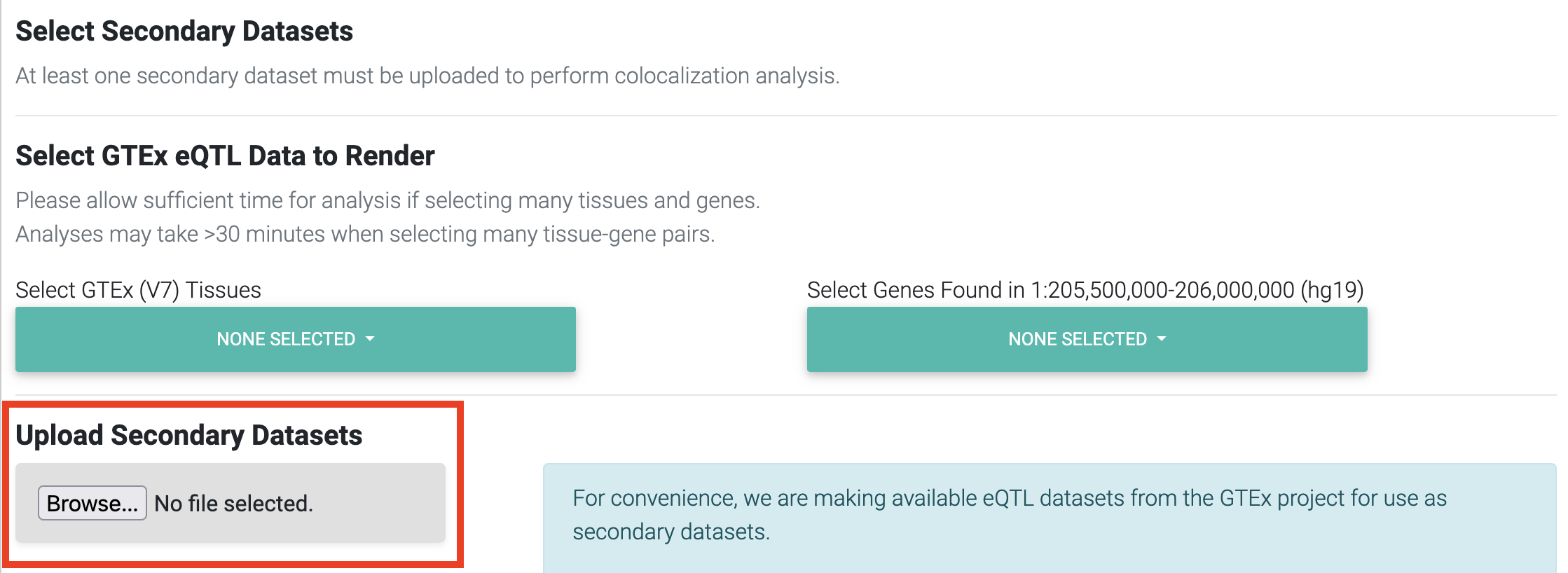
Upload button for uploading your secondary dataset(s)
In order for LocusFocus to recognize a dataset as secondary and perform colocalization testing, you must format your dataset in HTML format. The HTML format allows several datasets to be merged in a single HTML file. We suggest each dataset be preceded by an <h3> tag with the description title of the dataset.
We provide a python script to simplify the generation of the merged HTML dataset. To run both Simple Sum and COLOC2, please use the merge_and_convert_to_html_coloc2.py script.
The first step in creating the HTML file is to create a tab-separated descriptor file containing the list of files to be merged together (first column). The second column (tab-delimited) may contain descriptions of the datasets. The remaining columns specify the column names for chromosome, basepair position, SNP name, P-value (in that order).
For example, suppose we had three genomewide association analyses (from Ben Neale) from the UK Biobank:
The first few lines for FVC look as follows:
> head 3062.assoc.mod.ROI.slc26a9.tsv

variant rsid    nCompleteSamples        AC      ytx     beta    se      tstat   pval    chr     pos     variant ref     alt
1:205860191:A:G rs149104610     307638  7.58684e+03     2.89852e+02     -1.06502e-02    9.01042e-03     -1.18199e+00    2.37211e-01     1       205860191       A       G
1:205860462:G:A rs183927606     307638  7.58336e+03     2.94623e+02     -1.03192e-02    9.01499e-03     -1.14467e+00    2.52347e-01     1       205860462       G       A
1:205860763:T:C rs182878528     307638  7.57953e+03     2.92349e+02     -1.04035e-02    9.01627e-03     -1.15386e+00    2.48558e-01     1       205860763       T       C
1:205860874:A:G rs573870089     307638  1.06676e+03     6.36134e+01     2.08202e-02     2.49968e-02     8.32914e-01     4.04894e-01     1       205860874       A       G
1:205861028:G:A rs36039729      307638  4.44225e+04     2.35233e+03     9.40215e-04     3.81097e-03     2.46713e-01     8.05131e-01     1       205861028       G       A
1:205861107:C:T rs9438396       307638  2.85296e+04     1.97301e+03     9.23118e-03     4.68786e-03     1.96917e+00     4.89347e-02     1       205861107       C       T
1:205861225:G:A rs115170053     307638  5.08637e+03     3.62211e+02     6.28049e-03     1.11434e-02     5.63607e-01     5.73022e-01     1       205861225       G       A
1:205861433:G:C rs6670490       307638  2.88292e+04     1.99373e+03     8.56608e-03     4.66254e-03     1.83721e+00     6.61794e-02     1       205861433       G       C
1:205862075:T:C rs6665183       307638  2.18993e+04     1.26147e+03     1.50666e-04     5.70059e-03     2.64299e-02     9.78914e-01     1       205862075       T       C
Note that we modified the original file by adding the chromosome and position columns
The FEV1 and PEF phenotype association files look similar.
To merge the summary statistics from these three files into a merged HTML file, we would first create a descriptor file of all the files we would like to merge. See below for the case of combining these three files:
> cat slc26a9_uk_biobank_spirometry_files_to_merge.txt

3062.assoc.mod.ROI.slc26a9.tsv       Forced vital capacity (FVC) - 3062      chr     pos     rsid pval
3063.assoc.mod.ROI.slc26a9.tsv       Forced expiratory volume in 1-second (FEV1) - 3063      chr     pos     rsid    pval
3064.assoc.mod.ROI3.slc26a9.tsv      Peak expiratory flow (PEF) - 3064       chr     pos     rsid    pval
Each column (tab-separated) defines:
Filename
Description title
Chromosome column name
Basepair coordinate position column name
rs ID column name (alternatively, you may specify a column with variant ID formatted as chrom_pos_ref_alt_b37; e.g. 1_205860191_A_G_b37)
P-value
Note that COLOC2 assumes an eQTL dataset as secondary input, and the merge_and_convert_to_html_coloc2.py script must be used, which requires the same inputs as above, plus the following:
Beta
Standard error
Number of samples
A1 (minor) or alternate allele
A2 (major) or reference allele
Minor allele frequency (MAF)
Probe ID
You may refer to the github page for more examples of datasets, where a sample descriptor file and sample command are provided for guidance to build a secondary dataset to also run COLOC2 colocalization.
While running COLOC2 is possible, we proceed below with the simpler example without COLOC2. The steps to also include COLOC2, however, are similar.
Then, to generate the merged html file while subsetting the region we may issue the command as follows:
> python3 merge_and_convert_to_html.py slc26a9_uk_biobank_spirometry_files_to_merge.txt 1:205860000-205923000 slc26a9_uk_biobank_spirometry_merged.html
A description of the positional arguments may be issued with the -h or –help arguments:
> python3 merge_and_convert_to_html.py -h

usage: merge_and_convert_to_html.py [-h]
   filelist_filename coordinates outfilename

Merge several datasets together into HTML tables separated by <h3> title tags

positional arguments:
   filelist_filename  Filename containing the list of files to be merged
                  together. The second column (tab-delimited) may contain
                  descriptions of the datasets. The remaining columns
                  specify the column names for chromosome, basepair
                  position, SNP name, P-value (in that order).
   coordinates        The region coordinates to subset from each file (e.g.
                  1:500,000-600,000
   outfilename        Desired output filename for the merged file

optional arguments:
   -h, --help         show this help message and exit
The above command will generate the merged slc26a9_uk_biobank_spirometry_merged.html, file which can be used with LocusFocus.
Some important points to consider
Please note that your GWAS and secondary datasets must be subset in order to reduce the file size for uploading purposes (current combined limit is 100 MB).
You must also enter the genomic location you are interested in the HG19 Coordinates field. The format must be chromosome:start-end, where start is the starting basepair position and end is the ending basepair position.
The region size entered in Coordinates field cannot be larger than 2 MBbp.
If the SNP column has multiple rsid’s separated by semicolon, the first rsid will be used.
The SNP rs id is not used for determining the presence of the SNP in the 1000 Genomes population for the LD calculation; the chromosome and position columns determine this. If the chromosome:position combination is found in the 1000 Genomes, then the pairwise LD will be calculated for that particular SNP.
The LD matrix is calculated for chromosome:position SNPs available in both GWAS input and the selected 1000 Genomes population datasets.
Only overlapping SNPs are used for the Simple Sum calculations, and only overlapping SNPs with the primary dataset are plotted.
A region within +/- 0.1 Mbp is selected around the top SNP to compute the Simple Sum p-value. This area is shaded gray in the first plot. This is done for each gene found within +/- 1 Mbp of the top SNP for all the tissues selected.
It is important to have a dense set of genotyped SNPs to get an accurate assessment of the Simple Sum p-value calculation.